Understanding the Variational Lower Bound

Introduction

Variational Bayesian (VB) Methods are a family of techniques that are very popular in statistical Machine Learning. One powerful feature of VB methods is the inference-optimization duality [1]: we can view statistical inference problems (i.e. infer the value of a random variable given the value of another random variable) as optimization problems (i.e. find the parameter values that minimize some objective function). Furthermore, the variational lower bound, also called evidence lower bound (ELBO), plays an essential role in the VB derivations. In this note, we aim to introduce the basic ideas of variational lower bound, which can help to understand the derivations of the learning rules in the papers related to “hard attention” mechanism [2], [3], [4], [5].

Variational Lower Bound

Problem setup

Assume that $X$ are observations (data) and $Z$ are hidden variables. Note that we are general – the hidden variables might include the “parameters”. The relationship of these two variables can be represented using the following graphical model.

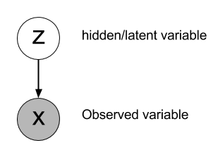
Moreover, uppercase $P(X) $ denotes the probability distribution over that variable, and lowercase $p(X)$ is the density function of the distribution of $X$. The posterior distribution of the hidden variables can then be written as follows using the Bayes’ Theorem.

$p(Z|X) = \frac{p(X|Z)p(Z)}{p(X)} = \frac{p(X|Z)p(Z)}{\int_Z p(X,Z)}$

First derivation: the Jensen’s inequality

Starting from the log probability of the observations (the marginal probability of $X$ ), we can have:

$\begin{aligned} \log p(X) &= \log \int_Z p(X,Z) \\ &= \log \int_Z p(X,Z) \frac{q(Z)}{q(Z)} \\ &= \log \left( \mathbb{E}_q\left[\frac{p(X,Z)}{q(Z)}\right] \right)\\ &\geq \mathbb{E}_q\left[\log \frac{p(X,Z)}{q(Z)} \right] \\ &= \mathbb{E}_q\left[\log p(X,Z)\right] + H[Z] \end{aligned}$

Equation (5) is the variational lower bound, also called ELBO.

The $q(Z)$ in equation (2) is a distribution we use to approximation the true posterior distribution $p(Z|X)$ in VB. For here, we can view it as an arbitrary distribution and the derivations still hold. Equation (4) applies the Jensen’s inequality $f\left(\mathbb{E}[X]\right) \leq \mathbb{E}\left[f(X) \right]$ for the concave log function. $H[Z] = -\mathbb{E}_q[\log q(Z)]$ is the Shannon entropy.

Let us denote:

$L = \mathbb{E}_q\left[\log p(X,Z)\right] + H[Z]$

Then it is obvious that $L$ is a lower bound of the log probability of the observations. As a result, if in some cases we want to maximize the marginal probability, we can instead maximize its variational lower bound $L$.

Second derivation: KL divergence

In the last section, we did not pay much attention on the distribution $p(Z)$. However, this distribution $p(Z)$ is actually the core motivation of the VB methods. In many cases, the computation of the posterior distribution $p(Z|X)$ is always intractable. For example, we need to integrate (sum up) all configurations of the hidden variables in order to computer the denominator.

The main idea behind variational methods is: to find some approximation distributions $q(Z)$ that are as closed as possible to the true posterior distribution $p(Z|X)$. These approximation distribution can have their own variational parameters: $q(Z|\theta)$, and we try to find the setting of the parameters that make $q$ close to the posterior of interest. Obviously the distribution $q(Z)$ should be relatively easy and more tractable for inference.

To measure the closeness of the two distribution $q(Z)$ and $p(Z|X)$, a common metric is the Kullback-Leibler (KL) divergence. The KL divergence for variational inference is:

$\begin{aligned} KL\left[q(Z) \| p(Z|X)\right] &= \int_Z q(Z) \log \frac{q(Z)}{p(Z|X)} \\ &= -\int_Z q(Z) \log \frac{p(Z|X)}{q(Z)} \\ &= - \left(\int_Z q(Z) \log \frac{p(X,Z)}{q(Z)} - \int_Z q(Z) \log p(X)\right) \\ &= -\int_Z q(Z) \log \frac{p(X,Z)}{q(Z)} + \log p(X) \int_Z q(Z) \\ &= -L + \log p(X) \end{aligned}$

where $L$ is the variational lower bound defined above. Equation (10) is obtained by the normalization constraint: $\int_Z q(Z) = 1$. Rearrange the equations we can get:

$L = \log p(X) - KL\left[q(Z) \| p(Z|X)\right]$

As KL divergence is always $\geq 0$, once again we get $L \leq \log p(X)$ is a lower bound of the log probability of observations. And we also know the difference between them is exactly the KL divergence of the approximation and true distribution. In others words, the lower bound L hits the log probability iff the approximation distribution is perfectly closed to the true posterior distribution.

Example

Multiple Object Recognition with Visual Attention

Now, we can use our understanding of the variational lower bound to deduce the learning rules in practical problems. We use the paper [2] as an example.

First of all, we want to maximize the log likelihood of the class label: $\log p(y|I, W)$. Here $I$ is the image, $W$ is the model parameters and $y$ is the class label, which can be viewed as an observable variable. Then, the objective function above can be rewritten by marginalizing over the locations $l$ (hidden variables):

$\log p(y|I,W) = \log \sum_l p(l|I,W)p(y|l,I,W)$

We can obtained its lower bound directly using Jensen’s inequality:

$\log \sum_l p(l|I,W)p(y|l,I,W) \geq \sum_l p(l|I,W) \log p(y|l,I,W)$

We can also get the same result using the variational lower bound of the marginal probability of observations and setting $q(l) = p(l|I,W)$:

$\log p(y|I,W) \geq \sum_l q(l) \log\frac{p(y,l|I,W)}{q(l)} = \sum_l p(l|I,W) \log p(y|l,I,W)$

Then, we can maximize the variational lower bound instead by taking derivatives of it with respect to the model parameter $W$. Almost the same derivations are also used in [@xu2015show].

Conclusion

In this note, we introduce what variational lower bound is and its role in VB methods. We deduce the variational lower bound in two different ways and provide clear ideas about its relationship with other entities. We also go through a concrete exampling showing how to use the variational lower bound to obtain practical learning rules, which is very useful for understanding related papers.

Acknowledgement

This note is a reading note that borrows many ideas from the following papers or posts: [1], [6], [7], [8], [9].

Reference

[1] E. Jang. A Beginner’s Guide to Variational Methods: Mean-Field Approximation. http://blog.evjang.com/2016/08/variational-bayes.html, 2016.

[2] J. Ba, V. Mnih, and K. Kavukcuoglu. Multiple object recognition with visual attention. arXiv preprint arXiv:1412.7755, 2014.

[3] T. Lei, R. Barzilay, and T. Jaakkola. Rationalizing neural predictions. EMNLP, 2016.

[4] K. Xu, J. Ba, R. Kiros, K. Cho, A. C. Courville, R. Salakhutdinov, R. S. Zemel, and Y. Bengio. Show, attend and tell: Neural image caption generation with visual attention. In ICML, volume 14, pages 77–81, 2015.

[5] V. Mnih, N. Heess, A. Graves, et al. Recurrent models of visual attention. In Advances in neural information processing systems, pages 2204–2212, 2014.

[6] D. M. Blei. Variational inference. Lecture from Princeton, variational inference, 2011.

[7] C. W. Fox and S. J. Roberts. A tutorial on variational bayesian inference. Artificial intelligence review, pages 1–11, 2012.

[8] D. G. Tzikas, A. C. Likas, and N. P. Galatsanos. The variational approximation for bayesian inference. IEEE Signal Processing Magazine, 25(6):131–146, 2008.

[9] Z. Ghahramani. Variational methods. Lecture from CMU, Statistical Approaches to Learning and Discovery, 2003.